Introduction

In this document we describe the On-The-Fly (OTF) observing system of the ASTE. See Sawada et al. 2008, PASJ, 60, 445 (arXiv:0712.1283) for details.

OTF is a technique to perform mapping observations: the antenna is driven continuously in a mapping region and the data are taken in short interval (0.1 second in case of ASTE). The OTF observations have advantages over usual position-switch observations as follows. OTF is effective in particular when a wide area is surveyed in relatively short integrations.

dead time of the telescope reduces (see the next section).
the system variation (e.g., atmospheric conditions, pointing of the telescope) does not affect the map since the entire map can be scanned in a short period.
since the data are aquired more frequently than the Nyquist sampling rate, the spatial information is not lost.

Also see documents listed below.

Mangum, Emerson, & Greisen 2007, A&A, 474, 679 (ADS)
Kitt Peak 12-m: http://www.cv.nrao.edu/~jmangum/12meter/docs/otfdoc.ps
FCRAO 14-m: http://donald.astro.umass.edu/~fcrao/library/manuals/otfmanual.html
IRAM 30-m: http://iram.fr/IRAMES/groups/astronomy/OTF/HTML/sl-otf.html
SMTO 10-m: http://www.mpifr-bonn.mpg.de/div/hhertz/smto-otf-guide/smto-otf-guide.html

Though raster-scan observations of radio continuum is also a kind of OTF, we describe OTF spectral line observations in this document.

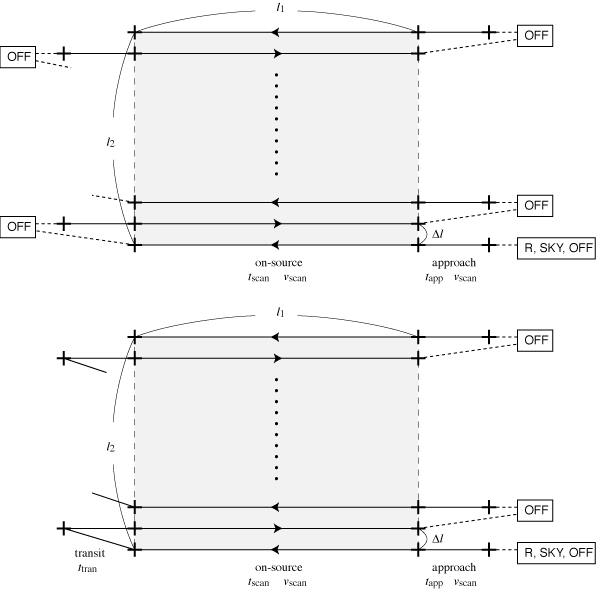
Schematic illustration of an OTF scan pattern is shown in Fig. 1-1. The behavior of the antenna is similar to those in raster mapping of continuum observations. The "on-source" part of the figure stands for the main-run of a scan (hereafter simply "scan"), during which the antenna is driven at a constant speed and the data are taken at every 0.1 (ACG) or 0.2 (WHSF) second. The "approach-run" is inserted before every scan to let the antenna move stably during the scan. If there is no OFF (integration on emission-free reference position) between two scans (Fig. 1-1 bottom), a "transit-run" (from the end point of the first scan to the start point of the second scan) is inserted. We recommend to set the approach and the transit to be 4 seconds and 2 seconds, respectively. (see Development and Evaluation of ASTE OTF).

Like usual position switch ("step-and-integrate") observations, the "chopper-wheel" calibration (R-SKY) data should be obtained during the observation in an appropriate interval. OFF points are taken before every scan or several scans.

Fig. 1-1: scan pattern
Fig. 1-1: Schematic illustration of an OTF scan pattern. (top) in case of a sequence pattern of "1*" (OFF-ON); (bottom) in case of a sequence pattern of "1**" (OFF-ON-ON).

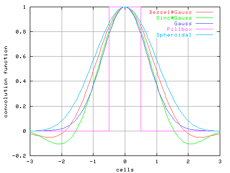
As a result of the observations, the mapped region is filled with (spectrum) data points with spacings smaller than the Nyquist sampling rate. Since the data points do not align on any regular grid, the data should be regridded onto a regular grid using a convolution funciton. Convolution functions implemented are as follows (Fig. 1-2):

Gaussian-tapered 1st-order Bessel function
$\frac{J_1(r/a)}{r/a} \times \exp\left[ -\left( \frac{r}{b} \right)^2 \right]$
where r is the distance between the grid point and the spectrum data point [pixels], a=1.55/ $\pi$ , b=2.52. See also "Miscellaneous Information".
Gaussian-tapered Sinc function
$\frac{\sin (r/a)}{r/a} \times \exp\left[ -\left( \frac{r}{b} \right)^2 \right]$
where r is the distance between the grid point and the spectrum data point [pixels], a=1.55/ $\pi$ , b=2.52.
Gaussian
$\exp\left[ -\left( \frac{r}{a} \right)^2 \right]$
where r is the distance between the grid point and the spectrum data point [pixels], a=1.
Pillbox (Cell-averaging)
$1 (|x| \le 0.5, |y| \le 0.5), 0 \mbox{(otherwise)}$
where x, y are offsets from the grid point and the spectrum data point along X and Y directions [pixels], respectively.
These 4 functions described above are taken from Mangum (1999); Mangum, Emerson, & Greisen (2000).
Spheroidal function
$|1-\eta_x^2|^\alpha \psi_{\alpha 0}(c,\eta_x)\cdot |1-\eta_y^2|^\alpha \psi_{\alpha 0}(c,\eta_y) (|\eta_x|\le 1, |\eta_y|\le 1), 0 \mbox{(otherwise)}$
where x, y are offsets from the grid point and the spectrum data point along X and Y directions [pixels], respectively, and $\eta$ _x = 2x/m, $\eta$ _y = 2y/m. See Schwab (1984) for details.
In the Map GUI, specify Schwab's two parameters: m(=4,5,6,7,8) and $\alpha$ (=0.0,0.5,1.0,1.5,2.0).

Fig. 1-2: Convolution functions implemented so far; Bessel*Gauss (a=1.55/ $\pi$ , b=2.52), Sinc*Gauss (a=1.55/ $\pi$ , b=2.52), Gauss (a=1.0), Pillbox, and Spheroidal (m=6, $\alpha$ =1.0).

last update: 2008-06-26