Determining parameters for OTF observations

Conceptual diagram of OTF scan

Figure 1 shows the scan patterns of OTF observations. In Figure 1, "on-source" represents the main scan (hereafter we call "scan"), where the antenna moves with a constant velocity, v_scan, and records spectral data every t_dump (0.1 sec for MAC, 0.2 sec for WHSF).

As in the case of position switch ("step-and-integration") observations, "chopper-wheel" calibration (R-SKY) data should be taken at the beginning and in the middle of observations. OFF position is observed every scan or several scans.

In order that the antenna points the specified direction stably during scans, "approach" comes before each scan. When an OFF position is not observed between scans (lower panel in Figure 1), "transit" is inserted between the end position and the start position. The above is the same as the continuum raster-scan observations. We recommend to set t_app = 4 sec for approach and t_tran = 2 sec for transit.

Fig. 1: scan pattern
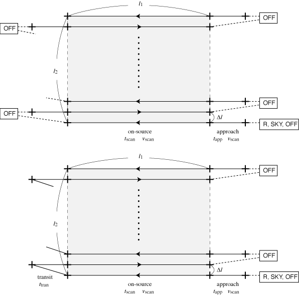
Figure 1: OTF scan pattern.
upper: Observing sequence "1*" (OFF-ON)
lower: Observing sequence "1**" (OFF-ON-ON).

Parameter determination and sensitivity estimate

The nominal observing efficiency increases with increase in t_scan (decrease in v_scan).

Parameters

assuming the observing area of l₁ ["] $\times$ l₂ ["] (l₁ in the direction of scan and l₂ in the vertical direction).
When the time needed for a scan (on-source) is t_scan [s], the scan velocity in the sky is v_scan ["/s] = l₁/t_scan.
t_scan should be set in order that the antenna slew length during the integration time t_dump [s] (0.1 sec for MAC and 0.2 for WHSF), t_dumpv_scan ["] does not exceed 1/3 or 1/4 of the beam width. For example, at 350 GHz, v_scan $\lsim$ 60 ["/s] for MAC and v_scan $\lsim$ 30 ["/s] for WHSF.
We assume the number of scans per OFF position is N_scan^SEQ, the spacing between scans is ${\mit\Delta}$ l ["], and the map grid size is d ["] $\times$ d ["]. ${\mit\Delta}$ l is set to about 1/3 of the beam width, and d is set to from about 1/3 to 1/2 of the beam width (d can be changed to some extent when data reduction). In this case, the number of scan is N_row = l₂/ ${\mit\Delta}$ l +1.

Sensitivity estimate

By using the setup above, the parameters are determined and the sensitivity is estimated as follows. (script for this is here: (otfaste.c / otfaste.pl).

Overhead time for a scan t_OH [s] is t_OH = 6 + 8/N_scan^SEQ
The integration time for OFF position is determined as follows:
$t_{\rm OFF} = \sqrt{\left(t_{\rm scan}+t_{\rm OH} \right) \frac{\eta N_{\rm scan}^{\rm SEQ} d t_{\rm scan}}{l_1}}$
where $\eta$ = 4.3 (note that this depends on the type of convolution function and parameters for map making. 4.3 for Bessel x Gauss, 1.2 for Sinc x Gauss, 6.3 for Gauss, 1.0 for Pillbox, and 10.2 for Spheroidal. Please see Sawada et al. 2008 for details.)
Total observing time including OFF positions and antenna slew time is
$t_{\rm OBStot} = N_{\rm row} \left(t_{\rm scan} + t_{\rm OH} + \frac{t_{\rm OFF}}{N_{\rm scan}^{\rm SEQ}} \right) f_{\rm cal}$
where f_cal is overhead time for R-SKY calibrations. When observing R-SKY for one minute per 15 minutes, f_cal is 16/15. When t_OBStot exceeds the time interval for pointings, observations are needed to be divided into multiple observing tables to reduce the observing time per observing table.
Total on-source scan time is
$t_{\rm ONtot} = N_{\rm row}t_{\rm scan} \simeq \frac{l_1 l_2}{{\mit\Delta}l \cdot v_{\rm scan}}$
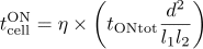
Integration time for ON positions and OFF positions per 1 grid (d $\times$ d) of the map is
$t_{\rm cell}^{\rm ON} = \eta \times \left( t_{\rm ONtot} \frac{d^2}{l_1 l_2} \right)$
$t_{\rm cell}^{\rm OFF} = t_{\rm OFF} \left( 1+\frac{d-{\mit\Delta}l}{N_{\rm scan}^{\rm SEQ}{\mit\Delta}l} \right)$
The rms noise temperature of the map is
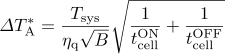
${\mit\Delta}T_{\rm A}^* = \frac{T_{\rm sys}}{\eta_{\rm q}\sqrt{B}}\sqrt{\frac{1}{t_{\rm cell}^{\rm ON}}+\frac{1}{t_{\rm cell}^{\rm OFF}}}$
where T_sys [K] is the system noise temperature, B [Hz] is the frequency resolution of the map, and $\eta$ _q is the quantization efficiency (0.88 for MAC and 0.64 for WHSF).

Hints for parameter selection

The nominal observing efficiency increases with increase in t_scan (decrease in v_scan). The upper limit on t_scan is determined by the following two factors:
- data (baseline) degrades with increase in the time interval between ON and OFF positions
- map becomes non-uniform with increase in observing time to cover the entire map area
The lower limit on t_scan is determined by the condition that t_dumpv_scan ["] should not exceed 1/3 or 1/4 of the beam width to prevent the beam smearing.
In map making, map is convolved with the width which corresponds to the grid size d. Therefore, if d is too small, the effective integration time (t_cell) decreases, and the noise level increases. This causes oversampling because the angular resolution is determined by the telescope beam size. If d is too large, the effective angular resolution increases (Figure 2).
Scanning in only one direction makes the scanning effect. Scanning in two directions that intersect at right angles and performing basket-weaving improve the scanning effect. The reduction software implements the method of PLAIT by Emerson & Gräve (1988). In case of scans with only one direction, the reduction software also implements the algorithm of PRESS by Sofue & Reich (1979).

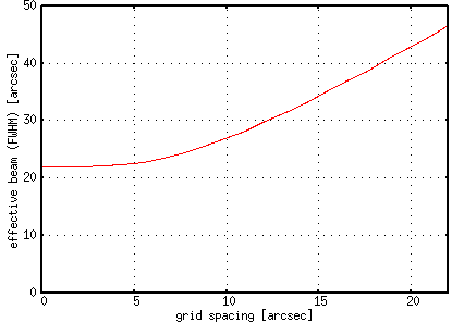
Fig. 2: FWHM growth against the grid spacing
Figure 2: Effective beam width (FWHM) as a function of grid spacing d.
When d is small, the effective beam width is close to the telescope beam width (assuming a Gaussian with a FWHM of 22").
When d is large, the effective beam width becomes asymptotic to the width of the convolution function $\simeq$ 2d.

Example

When using MAC with l₁=l₂=300 ["]、 t_scan=30 [s]、 ${\mit\Delta}$ l=7.5 ["]、 d=7.5 ["]、 T_sys(SSB)=500 [K]、 B=1 [MHz]

% perl otfaste.pl.txt
### OTF sensitivity estimation for ASTE ###
backend type                            (1:MAC, 2:WHSF): 1
length of mapping area (along the scans)    l1 [arcsec]: 300
length of mapping area (perp. to the scans) l2 [arcsec]: 300
time for scan                                 tscan [s]: 30
number of ONs per OFF                        Nscan(SEQ): 1
separation between scans              (delta)l [arcsec]: 7.5
map grid                                     d [arcsec]: 7.5
system noise temperature                       Tsys [K]: 500
resolution bandwidth                            B [kHz]: 1000
----------------------------------------------------------------
vscan=10.0["/sec] (1.0" per 0.1s sample)
tOFF=12.1[s] -> 12[s]
tOH=14.0[s]
ttot(ON)=20.5[min]
ttot(OBS)=40.8[min]
eta(ON/OBS)=0.50
tcell(ON)=3.31[s]
tcell(OFF)=12.00[s]
dTa*=0.35[K]

The optimum integration time for OFF position is 12 sec, ${\mit\Delta}$ T_A^*=0.35 [K] with the observing time of 40 minutes, and the effective angular resolution is 24".

# Tips: Redirection by using a parameter file (otfaste_input.txt) perl otfaste.pl.txt < otfaste_input.txt is easer for recalculations.