Observations

Making "Observe Table"

Source Table

Same as normal observations. Refer to Source Table sections of the aobs manual. Observations of the solar system objects do not work so far.

Open "Scan Table (Line)" panel (Fig. 3-1). "Off/Calib Positions", "Sequence", and "Calibration" are analogous with those of normal observations (please set the same coordinate systems for "On Positions" and "Off/Calib Positions"). Set the integration time for R-SKY calibration to about the same value as the OFF point integration.

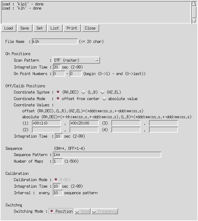
Fig. 3-1: Scan Table window of aobs.

Select "OTF (raster)" from "Scan Pattern" menu, then Scan Pattern window (Fig. 3-2) appears. Specify parameters listed below. Refer to Scan Table (Line/OTF) section of the aobs manual.

Coordinate System: Specify reference coordinate system. Should be (RA,DEC) or (L,B). Note that (AZ,EL) does not work.
Scan
- dX0, dY0: Relative coordinate of start position of the first scan.
- Direction: Direction of the scans.
- Length: Length of scans (l₁).
- Spacing: Spacing between the scans. ( ${\mit\Delta}$ l).
- Begin - End: Begin and end number of scan rows.
- Position Angle: Position angle between the XY coordinates from the reference coodinates
Time
- Approach: Duration of approach-run (t_app). We recommend to set this parameter to be 4 seconds.
- Scan: Duration of scan (main-run) (t_scan).
- Transient: Duration of transit-run (t_tran). We recommend to set this parameter to be 2 seconds.
- Return: Duration to return-run from the end point of the last scan to the start point of the first scan.

Fig. 3-2: Scan Pattern (OTF)
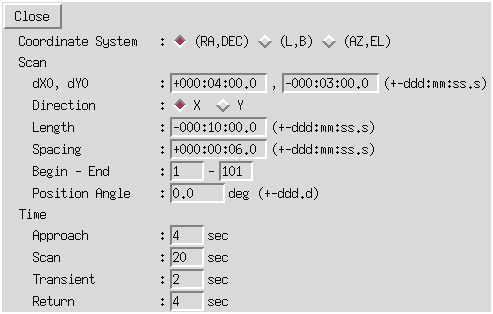
Fig. 3-2: Scan Pattern window.

Device Table

Same as normal observations. Refer to Device Table (Line) sections of the aobs manual.

Verifying the Table

With a shell script obspointotf.sh, scan paths of OTF tables can be plotted. Gnuplot and awk are required to use the script. (If awk is a too primitive version, the script will not work correctly. In that case, set full path to somewhat newer awk/nawk/gawk in a variable AWK instead of AWK=`which awk`: e.g., AWK=/home0/opt/bin/awk .) Usage is as follows:

obspointotf.sh [-ps/-cps] [-out] [-lp] [-xr Xblc:Xtrc] [-yr Yblc:Ytrc] infile1 [infile2 ...]

When you "Make" or "Send" an observe table, a file TableName.start is created in the directory /home/GROUP/PROJECT/obstable/ . Specify this ".start" file (or files) as an argument of obspointotf.sh to plot scan paths. You can close the plot window by typing "q" key when the window is focused.

cd /home/GROUP/PROJECT/obstable
obspointotf.sh hoge.start fuga.start

An option -ps is used to write monochrome PostScript onto the standard output. Use -cps for color PostScript.

obspointotf.sh -ps hoge.start | lpr
obspointotf.sh -cps hoge.start > hoge.ps

With the -out option, a temporal file "_ObsPointOtf_tmp_file.dat" is retained in the current directory. The "with linespoints" style of gnuplot is applied by setting the -lp option, otherwise "with lines" style is used.

Using -xr and/or -yr, a region to be plotted can be specified.

obspointotf.sh -xr 10:5 -yr -10:-5 hoge.start

Executing Observations

Just like as normal observations, select a observe table and press "Start Observation" to run the observation.

A line profile averaged in a specified duration is displayed in QLOOK. The time to average spectra can be set in the Device Table. The default is 5 seconds. This value is also the interval of the quick-merge data. QLOOK works in the same way as normal line observations ("Integration mode" does not work).

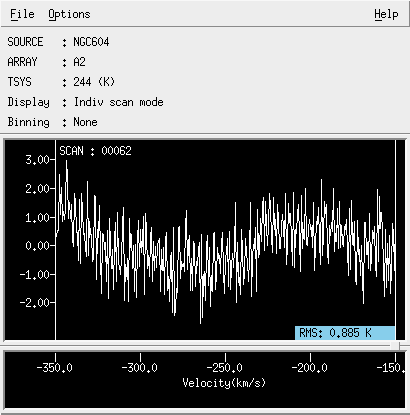
Fig. 3-3: OTF QLOOK.

last update: 2008-06-01